Exploratory Data Analysis (EDA) of IMDB Dataset

This post dives into an Exploratory Data Analysis (EDA) of a publicly available IMDB dataset. We’ll explore the characteristics of data and perform preprocessing steps to prepare it for further analysis.

Code examples and final results are valuable via Colab, Kaggle, and Github. this post focuses on a step-by-step approach to performing EDA on an IMDB dataset, outlining the thought process behind each step in my workflow.

All cells containing interactive visualizations that are hard to explore via images are are linked to the Google Colab Notebook via Icon. However to present this type of data to stakeholders make sure to use Data Story Telling techniques, tables, and highlights to deliver better results.

Introduction

Exploratory Data Analysis (EDA) is the cornerstone of data analysis. It’s where we leverage statistical techniques and visualizations to unearth the hidden structure, patterns, and anomalies within a dataset.

This post delves into an EDA of the IMDB dataset, a goldmine of information on movies, TV shows, and industry professionals. Our focus goes beyond just the results; we’ll explore the meticulous step-by-step process of uncovering insights and tackling challenges along the way.

We’ll delve into identifying and resolving common issues encountered with the IMDB dataset, offering practical tips for efficient data manipulation using Pandas and Plotly.

Data Acquisition and Overview

This section focuses on acquiring and describing the IMDB dataset. We’ll get a high-level understanding of its structure, content, and potential quality issues.

Information courtesy of IMDb. Used with permission.
Non-Commercial Licensing

First look at dataset

The IMDB dataset can be downloaded via it’s dataset page and consists of several tab-delimited files (TSV) compressed with gzip (.gz extension). While many datasets don’t come with a Data Dictionary or documentation, a short summery of IMDB dataset is available in IMDB Interfaces.

Here’s a breakdown of the files and their contents:

title.basics.tsv.gz: Contains information on movies, TV series, and other media items (tconst is the indexing key).
title.ratings.tsv.gz: Stores media rating data (likely linked to tconst in title.basics.tsv.gz).
title.akas.tsv.gz: Provides alternative titles for media items across languages and regions (relates to tconst in title.basics.tsv.gz with a one-to-many relationship).
title.episode.tsv.gz: Lists episodes for TV shows and series (relates to tconst in title.basics.tsv.gz with a one-to-many relationship).
name.basics.tsv.gz: Provides basic profiles for people (nconst is the indexing key).
title.crew.tsv.gz: Lists writers and directors (likely linked to tconst in title.basics.tsv.gz).
title.principals.tsv.gz: Details cast and crew members with their roles (many-to-many relationship with name.basics.tsv.gz).

Based on the filenames and provided information, we can infer the following relationships between the files:

title.basics.tsv.gz and title.ratings.tsv.gz: One-to-one (mergeable by tconst).
title.basics.tsv.gz and title.akas.tsv.gz, title.episode.tsv.gz: One-to-many (tconst is the foreign key).
title.basics.tsv.gz and title.crew.tsv.gz: One-to-one.
title.crew.tsv.gz and name.basics.tsv.gz: Many-to-many.
name.basics.tsv.gz and title.principals.tsv.gz: Many-to-many.

Key(index) columns:

tconst Indexing key for media items(movies, tv series, episodes, …).
nconst Indexing key for people(cast, crew, writers, …)

Opening the file in a text reader, I noticed that it’s tab separated(.tsv extension of files was also an indicator of this), and that they have a header row, so there is no need to ask the csv_reader to avoid skipping it.

Libraries

We’ll utilize Pandas for data manipulation and exploration throughout this project. Seaborn, Plotly will be used for data visualization. So they must be imported. Also as the project progresses, we’ll add any further libraries, imports, function, and variables we’ll globally need to this section.

# Importing Libraries
import os, csv
import pandas as pd
import numpy as np
import seaborn as sns
import matplotlib.pyplot as plt
import plotly.express as px
import plotly.graph_objects as go
from plotly.subplots import make_subplots
from tqdm.auto import tqdm
from IPython.display import display

# Sample data
def display_sample(df,n=5):
  """Displays a sample of the dataframe, including head, tail, and a random sample.
  Args:
      df: The pandas dataframe to display a sample of.
      n: (Optional) The number of rows to include in the random sample
          (default: 5).
  """
  display(pd.concat([df.head(), df.sample(n=n), df.tail()]))

# Show unique values in specific columns of a dataframe
def show_unique_cols(df, columns):
  """Show unique values in specific columns inside a dataframe
  Args:
      df: The pandas dataframe.
      columns: A list of column names
  """
  uniuque_series = pd.Series({c: df[c].unique() for c in columns})
  for row in columns:
    print(f"Unique values for '{row}' row:\n{uniuque_series[row]}\n")

dir_path = "/content/Datasets/IMDB"

display_sample function: Most data scientists, in this stage, use Panda’s head() and tail() to see starting and finishing rows of a dataset, however I like to concatenate them with a random sample of dataset in the middle. It provides a more comprehensive initial view of the data.

show_unique_cols function: this functions can list all unique values in a column holding list of values, such as genre data.

Finally dir_path is used to set the directory used for download dataset and to locate it’s files.

Download & Extract Dataset

Since the IMDB dataset is publicly available for download, we’ll focus on the download and extraction steps within the code section.

# Download with progressbar
def download(url, path):
  import math
  import requests
  from tqdm.auto import tqdm

  r = requests.get(url, stream=True, allow_redirects=True)
  total_size = int(r.headers.get("content-length", 0))
  block_size = 1024
  with open(path, "wb") as f:
    for data in tqdm(r.iter_content(block_size), total=math.ceil(total_size // block_size), unit="KB", unit_scale=True, desc=f"Downloading `{url}`"):
      f.write(data)

# Download & Extract dataset if it doens't exist
def get_dataset(url, dir_path, file):
  import gzip, shutil

  file_path = os.path.join(dir_path, file)
  extracted_file, extracted_file_path = file[:-3], file_path[:-3] # -4 removes `.gz` from end of file
  # Setup Dataset Directory
  if not os.path.exists(dir_path):
    from pathlib import Path
    Path(dir_path).mkdir(parents=True, exist_ok=True)
  # Download compressed
  if not os.path.isfile(file_path):
    if os.path.exists(extracted_file_path):
      print(f"Extracted version of file(`{extracted_file}`) already exists, skipping to next download.")
    else:
      download(url, file_path)
  else:
    print(f"file `{file}` already exists, skipping to next download.")
  # Extract Compressed
  if not os.path.isfile(extracted_file_path):
    print(f"Extracting `{file}` into `{extracted_file}.")
    with gzip.open(file_path, 'rb') as f_in:
      with open(extracted_file_path, 'wb') as f_out:
        shutil.copyfileobj(f_in, f_out)
  else:
    print(f"file `{extracted_file_path}` already exists, skipping to next.")


# Setup download parameters
url = "https://datasets.imdbws.com/"
files = ["title.ratings.tsv.gz", "title.basics.tsv.gz", "name.basics.tsv.gz", "title.akas.tsv.gz", "title.crew.tsv.gz", "title.episode.tsv.gz", "title.principals.tsv.gz"]
# download files
for file in files:
  get_dataset(f"{url}{file}", dir_path, file)

Initial Data Exploration on `title.basics.tsv.gz`

Since this dataset consist of multiple files we can check each of them. We’ll start by reading the title.basics.tsv.gz file using Pandas, seeing it’s information, and finally a displaying a sample of data.

# Reading the file
path = os.path.join(dir_path, "title.basics.tsv")
media_df = pd.read_csv(path, sep='\t', low_memory=False)

# DataFrame information & Sampling
media_df.info()
display_sample(media_df)

Note that encoding="utf-8" parameter may be required in some operating systems.

This code helps us discover best column types and have a general idea of what the data we’ll be working with. however as we can see in further steps it’s not enough to determine if we’re reading data cleanly.

<class 'pandas.core.frame.DataFrame'>
RangeIndex: 10611247 entries, 0 to 10611246
Data columns (total 9 columns):
 #   Column          Dtype 
---  ------          ----- 
 0   tconst          object
 1   titleType       object
 2   primaryTitle    object
 3   originalTitle   object
 4   isAdult         object
 5   startYear       object
 6   endYear         object
 7   runtimeMinutes  object
 8   genres          object
dtypes: object(9)
memory usage: 728.6+ MB

	tconst 	titleType 	primaryTitle 	originalTitle 	isAdult 	startYear 	endYear 	runtimeMinutes 	genres
0 	tt0000001 	short 	Carmencita 	Carmencita 	0 	1894 	\N 	1 	Documentary,Short
1 	tt0000002 	short 	Le clown et ses chiens 	Le clown et ses chiens 	0 	1892 	\N 	5 	Animation,Short
2 	tt0000003 	short 	Pauvre Pierrot 	Pauvre Pierrot 	0 	1892 	\N 	4 	Animation,Comedy,Romance
3 	tt0000004 	short 	Un bon bock 	Un bon bock 	0 	1892 	\N 	12 	Animation,Short
4 	tt0000005 	short 	Blacksmith Scene 	Blacksmith Scene 	0 	1893 	\N 	1 	Comedy,Short
2707210 	tt1317524 	tvEpisode 	Pussy Boy 	Pussy Boy 	0 	2008 	\N 	\N 	Comedy
678585 	tt0701624 	tvEpisode 	Verlorener Sohn 	Verlorener Sohn 	0 	2005 	\N 	\N 	Crime
3851920 	tt1529028 	tvEpisode 	Goldfish Gulp 	Goldfish Gulp 	0 	2009 	\N 	\N 	Animation,Game-Show
1725515 	tt11366472 	tvEpisode 	Episode #1.220 	Episode #1.220 	0 	\N 	\N 	\N 	Drama
9665800 	tt7857842 	movie 	Trinity Gold Rush 	Trinity Gold Rush 	0 	2018 	\N 	\N 	Drama
10611242 	tt9916848 	tvEpisode 	Episode #3.17 	Episode #3.17 	0 	2009 	\N 	\N 	Action,Drama,Family
10611243 	tt9916850 	tvEpisode 	Episode #3.19 	Episode #3.19 	0 	2010 	\N 	\N 	Action,Drama,Family
10611244 	tt9916852 	tvEpisode 	Episode #3.20 	Episode #3.20 	0 	2010 	\N 	\N 	Action,Drama,Family
10611245 	tt9916856 	short 	The Wind 	The Wind 	0 	2015 	\N 	27 	Short
10611246 	tt9916880 	tvEpisode 	Horrid Henry Knows It All 	Horrid Henry Knows It All 	0 	2014 	\N 	10 	Adventure,Animation,Comedy

Here we can see a couple of issues which should be solved. For example:

NA values are shown as \N and if you look at the raw file in an editor you’ll see that \\N string is used.
Some columns such as startYear, endYear, and runtimeMinutes should be integers.
isAdult column represents a binary and should be integer(preferably 8-bit).
genres column is a list that is represented as a comma separated string. If we want to perform analysis on this column we should convert it from string into a list type.
Now let’s take a look at unique values of specific rows that should have a limited number of values:

uniuque_cols = ['titleType', 'isAdult', 'startYear', 'endYear', 'runtimeMinutes', 'genres']
show_unique_cols(media_df, uniuque_cols)

here we can see a number of issues with our data that should be solved. For example “Documentary,Reality-TV” should not be in runtimeMinutes column. this is normally done as a part of Data Cleaning task which is a part of Data Pre-Processing workflow. however I can see that there should be only a couple of rows that cause this. so I can detect them and remove them or find another way.

Let’s take a closer look. This code will show all rows with none numeric values in runtimeMinutes column:

media_df['runtimeMinutes'] = media_df['runtimeMinutes'].replace("\\N", 0)
media_df[pd.to_numeric(media_df['runtimeMinutes'], errors='coerce').isna()]

We can see that primaryTitle and originalTitle are merged. I’ve used Vim to search for raw line of this rows, though you can use a file reader to read this specific files; it seems that rows with title column starting with quote mark(“) are causing this issue. Example:

tt10233364    tvEpisode    "Rolling in the Deep Dish    "Rolling in the Deep Dish    0    2019    \N    \N    Reality-TV

In this example because of quote mark, the string "Rolling in the Deep Dish "Rolling in the Deep Dish will be considered a single column’s value despite the tab separating them. So if we ignore quote mark in the reader, this should be resolved.

Given the issue in quote marks and memory considerations, the csv reader’s code should be re-written to resolve mentioned problems:

path = os.path.join(dir_path, "title.basics.tsv")
media_df = pd.read_csv(path, low_memory=False, dtype={4:pd.Int16Dtype(), 5:pd.Int16Dtype(), 6:pd.Int16Dtype(),7:pd.Int32Dtype()}, sep='\t', encoding="utf-8", na_values=['\\N'], quoting=csv.QUOTE_NONE)

changes:

We assigned dtype parameter to set column data types which will help with memory consumption and makes future data manipulation faster.
Setting na_values will change all raw \\N strings to NA.
finally quoting parameter will solve the merged column problem for titles starting with quote mark.

At this point we’ve performed initial exploration of one the files. We should repeat this step for all the files in the dataset to cleanly read them.

Data Preparation for EDA

Having explored the title.basics.tsv.gz file, we’ll proceed by reading all the files based on their relationships and perform any data cleaning and transformation that may be required for analysis phase.

Loading `title.basics.tsv.gz`

We’ll use Pandas’ read_csv function with similar parameters as before, specifying the appropriate file paths and parameters required for handling potential encoding issues.

path = os.path.join(dir_path, "title.basics.tsv")
media_df = pd.read_csv(path, sep='\t', encoding="utf-8", low_memory=False, dtype={4:pd.Int8Dtype(), 5:pd.Int16Dtype(), 6:pd.Int16Dtype(),7:pd.Int32Dtype()}, na_values=["\\N"], quoting=csv.QUOTE_NONE)

Preparing and Loading `title.crew.tsv` and `title.ratings.tsv`

Now we’ll focuses on the task of reading the remaining files based on their relationships, providing an example for a one-to-one case.

# Read Crew and Rating files.
path = os.path.join(dir_path, "title.crew.tsv")
crew_df = pd.read_csv(path, sep='\t', encoding="utf-8", low_memory=False, na_values=["\\N"])
path = os.path.join(dir_path, "title.ratings.tsv")
rating_df = pd.read_csv(path, sep='\t', encoding="utf-8", low_memory=False, na_values=["\\N"], dtype={1:pd.Float32Dtype(), 2:pd.Int32Dtype()})

Now two file’s must be merged with the title’s dataframe:

media_df = media_df.merge(crew_df,on='tconst').merge(rating_df,on='tconst')

We now have two dataframes that are no longer needed since they had been merged with media_df. It’s always a good practice to manage memory consumption, so we should delete them. This will require the use of list which is a peculiarity, as just deleting them won’t free up RAM.

# delete the old dataframe to release memory.
lst = [crew_df, rating_df]
del crew_df, rating_df
del lst

As we have a binary column with ones and zeros, we can transform them to True and False values:

media_df['isAdult'] = media_df['isAdult'].map({0: False, 1:True})

now using media_df.info() and by sampling it, we can take another look at our data. It seems that the final transformation needed is changing genre, directors, and writers columns. for example "Documentary,Short" should be transformed into a this list: ['Documentary', 'Short']. This will be useful if we want to analyze frequencies such as most popular genre or find most prolific actors or directors.

media_df['genres'] = media_df['genres'].str.split(',')
media_df['directors'] = media_df['directors'].str.split(',')
media_df['writers'] = media_df['writers'].str.split(',')

Loading `title.episode.tsv`

We follow the same workflow as the other files to read remaining files. it mostly consists of exploring raw data, reading it with correct parameters, and selecting columns and data types for this columns.

path = os.path.join(dir_path, "title.episode.tsv")
episode_df = pd.read_csv(path, sep='\t', encoding="utf-8", na_values=["\\N"], dtype={2:pd.Int32Dtype(), 3:pd.Int32Dtype()})

Loading `title.akas.tsv`

I’ve used two different ways of loading this files as it’s a large file and due to Limitation in my free Colab instance’s memory it’s not possible to load the entire file. This is the code to load the entirety of aka file:

path = os.path.join(dir_path, "title.akas.tsv")
# Read all file data
aka_df = pd.read_csv(path, sep='\t', encoding="utf-8", na_values=["\\N"], dtype={7:pd.Int8Dtype()}, quoting=csv.QUOTE_NONE, low_memory=False)
aka_df['isOriginalTitle'] = aka_df['isOriginalTitle'].dropna().map({0: False, 1:True})
aka_df['types'] = aka_df['types'].str.split('\x02')
aka_df['attributes'] = aka_df['attributes'].str.split('\x02')

title.akas.tsv file contains isOriginalTitle column which is converted to boolean. Also two columns (types and attributes) that are arrays and where converted to lists.

And here is the code to load selected columns:

path = os.path.join(dir_path, "title.akas.tsv")
# Read selected columns which are used (Memory-efficient)
aka_df = pd.read_csv(path, sep='\t', encoding="utf-8", na_values=["\\N"], usecols=["titleId", "region","language"], quoting=csv.QUOTE_NONE, low_memory=False)

Loading `name.basics.tsv`

Similar to title.akas.tsv file, name.basics.tsv we can load all columns:

path = os.path.join(dir_path, "name.basics.tsv")
# Read all columns
name_df = pd.read_csv(path, sep='\t', encoding="utf-8", na_values=["\\N"], dtype={2:pd.Int16Dtype(), 3:pd.Int16Dtype()})
name_df['primaryProfession'] = name_df['primaryProfession'].str.split(',')

Or load fewer columns, as we don’t need them for analysis:

path = os.path.join(dir_path, "name.basics.tsv")
# Read selected columns which are used (Memory-efficient)
name_df = pd.read_csv(path, sep='\t', encoding="utf-8", na_values=["\\N"], usecols=["nconst", "primaryName", "birthYear", "deathYear"], dtype={2:pd.Int16Dtype(), 3:pd.Int16Dtype()})

Read `title.principals.tsv`

This file is also too large to be worked on on a Free Colab instance. That’s why I won’t be performing ETA on this file, however this is how it can be individually loaded:

path = os.path.join(dir_path, "title.principals.tsv")
principals_df = pd.read_csv(path, sep='\t', encoding="utf-8", na_values=["\\N"], usecols=["tconst", "nconst", "category", "job"])

Note that title.principals.tsv and name.basics.tsv files had columns that we didn’t need. so we selected which columns should be added to dataframe.

Understanding the Data: Summary Statistics and Exploration

This phase delves deeper into the data using summary statistics and exploratory techniques. Our goal is to uncover patterns, trends, and potential issues within the dataset.

Here are some common approaches we’ll employ:

Summary Statistics:
- We’ll utilize Pandas functions like describe(), value_counts(), and potentially more specialized functions depending on data types (e.g., nunique() for number of unique values). These functions will provide insights into central tendency, distribution, and categorical variable composition.
Data Visualization:
- We’ll leverage libraries like Matplotlib, Seaborn, or Plotly to create informative visualizations (histograms, boxplots, scatter plots, etc.) These visualizations will help us identify patterns, outliers, and relationships between variables.
Findings and Insights:
- We’ll leverage summery statistics and visualization techniques to gain insights from data and answer questions we find interesting. For example we can find most popular genres, most loved movies, the most prolific directors and so on.

By combining these techniques, we can gain a comprehensive understanding of the data’s characteristics and prepare it for further analysis.

Media Types

Media Type Distribution

title_type_counts = media_df['titleType'].value_counts()

fig = go.Figure(data=[go.Pie(labels=title_type_counts.index, values=title_type_counts.values)])
fig.update_layout(title_text="Media Type Distribution")
fig.show()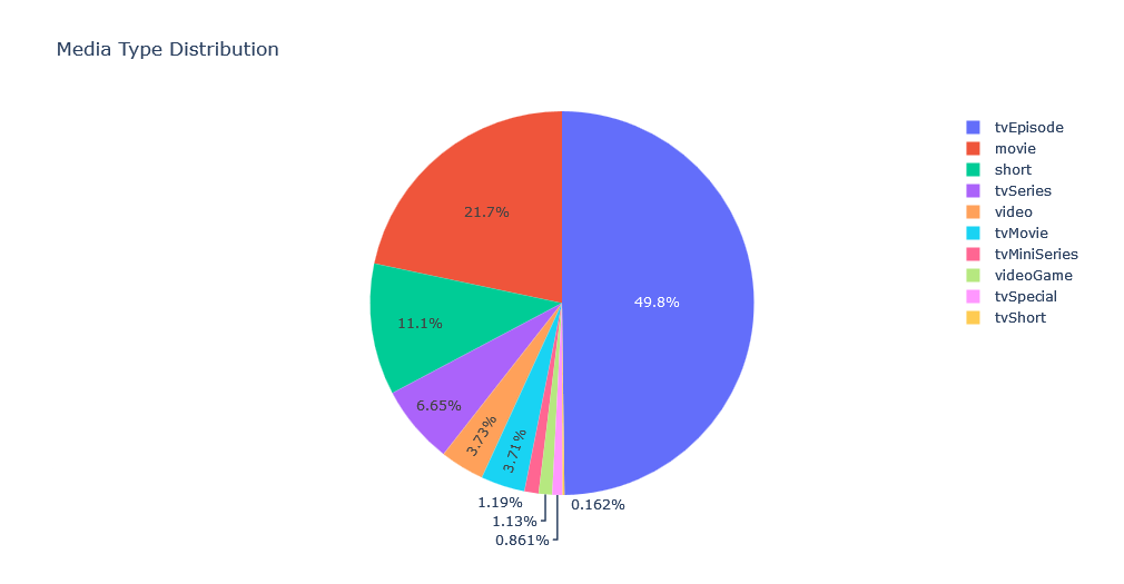

Genre

Genre WordCloud

from wordcloud import WordCloud

genre_frequencies = media_df['genres'].explode().value_counts()

wordcloud = WordCloud(width = 800, height = 400)
wordcloud.generate_from_frequencies(genre_frequencies)

plt.figure(figsize=(10, 5))
plt.imshow(wordcloud, interpolation="bilinear")
plt.axis('off')
plt.show()

Genres Frequency in a Bar Chart

# Simple bar chart plot to visualize the frequency of genres
genres = media_df['genres'].explode().value_counts().index.tolist()
genres_counts = media_df['genres'].explode().value_counts().values
df = pd.DataFrame({'genres': genres, 'genres_counts': genres_counts})

fig = px.bar(df, x="genres_counts", y="genres",height=700, orientation='h')
fig.show()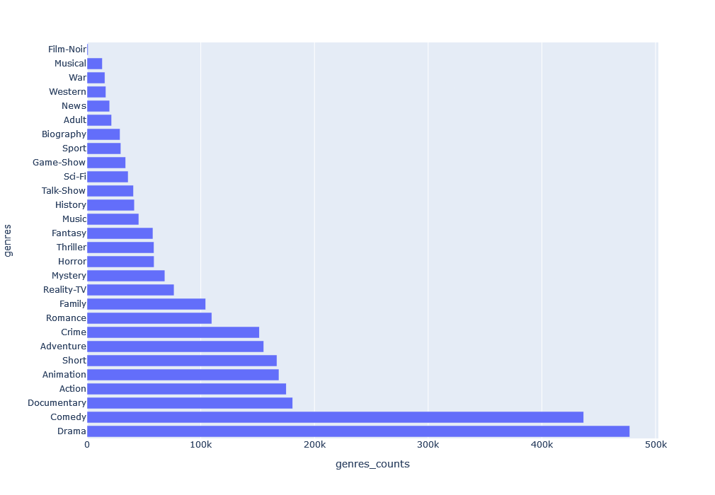

Genre Distribution Bar Chart in IMDB Dataset

Rating

Here, KDE Distribution of ratings using a histogram plot is visualized:

# KDE Distribution of ratings using a histogram plot
rating_mean, ratings_median = media_df.averageRating.mean(), media_df.averageRating.median()

plt.figure(figsize=(15,5))
ax = sns.histplot(media_df.averageRating, kde=True, color='skyblue')
ax.axvline(x=rating_mean,color=sns.color_palette("bright")[1],label=f"mean={rating_mean}")
ax.axvline(x=ratings_median,color=sns.color_palette("bright")[4],label=f"median={ratings_median}")

plt.legend()
plt.show()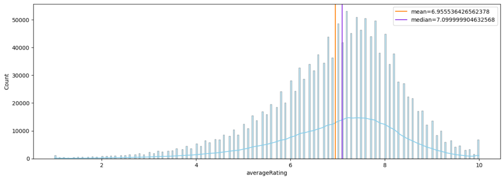

As you can see mean and media are marked in this plot using axvline() function of Seaborn histogram plot.

Score Analysis

Top 10 media with highest number of votes:

media_df.sort_values(by='numVotes', ascending=False).head(10)[['primaryTitle', 'startYear', 'numVotes', 'averageRating', 'genres']]

Top 10 highest rated movies with more than 10000 voters:

media_df[(media_df['numVotes'] > 10000) & (media_df['titleType']=="movie")].sort_values(by='averageRating', ascending=False).head(10)[['primaryTitle', 'numVotes', 'averageRating', 'genres']]

Top 10 Media through Sort:

media_df.sort_values(by=['numVotes', 'averageRating'], ascending=[False, False])[['primaryTitle', 'numVotes', 'averageRating', 'genres']].head(10)

Top 10 highest rated media, regardless of number of votes:

display(media_df.sort_values(by='averageRating', ascending=False).head(10)[['primaryTitle', 'runtimeMinutes', 'genres']])

If look at the results of past four analysis you can see that none of them can be used as a measure of a media’s true popularity. So we should look for better ways to rate the popularity of a media and there are many ways of doing it. However as data scientiest we should learn to work with data that we can get our hands on, and get the best insights we can with what we have got. To do so, given only number of votes and the rating, I’ve decided to use this method:

media_df['score'] = ((2 * media_df['averageRating'] - 11) / 9) * media_df['numVotes']
display(media_df.sort_values(by='score', ascending=False))

To calculate “score”, I’ve transformed “averageRating” from 1 to 10 into values into -1 to 1, then multiplied it with number of votes. This will give us a positive or negative number indicating how much an item is loved or hated.

Interestingly at the moment, Game of Thrones series is among top 5 medias, while it’s episode “The Iron Throne” us among top 10 hated media items.

Score Across Years

Now let’s visualize average score of movies across years

average_score_by_year = media_df[media_df['titleType'] == 'movie'].groupby('startYear')['score'].mean().reset_index()

fig = go.Figure()
fig.add_trace(go.Scatter(x=average_score_by_year['startYear'], y=average_score_by_year['score'], mode='lines+markers'))
fig.update_layout(title='Average Score Over the Years for Movies', xaxis_title='Year', yaxis_title='Average Score')

fig.show()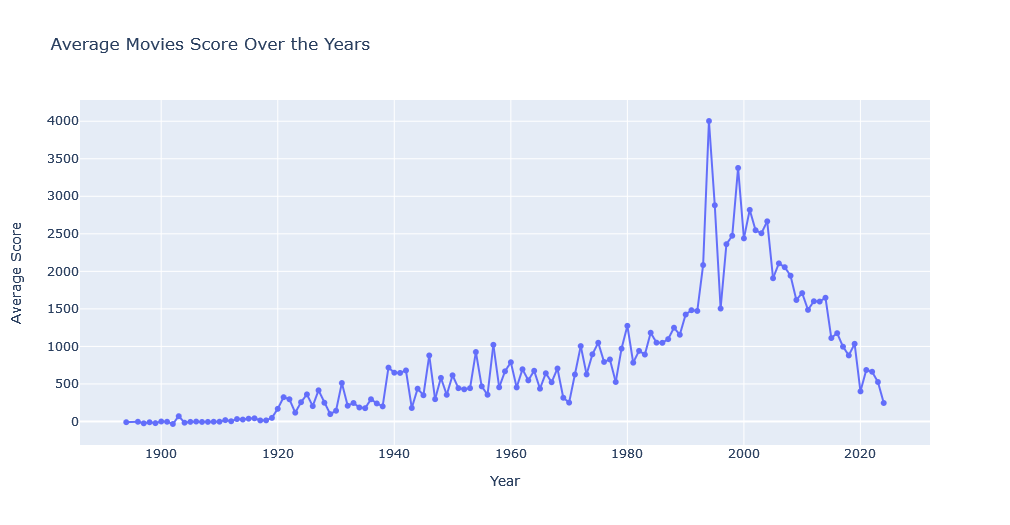

According to this graph, the movie industry peaked at 1994 and experienced another surge in 1999. However movies, as a whole, are more critically rated in past few years.

Run-Time

Media Runtime Distribution

Here we’ll visualize the distribution of media Run Time between 10 and 200 minutes (p.s. longest LOTR movie is 200 minutes). I’ve made this limitation because including the few media files that are too long will shrink the visualization and make it less usable.

filtered_runtime = media_df[(media_df['runtimeMinutes'] >= 10) & (media_df['runtimeMinutes'] <= 200)]['runtimeMinutes']

fig = go.Figure(data=go.Histogram(x=filtered_runtime))
fig.update_layout(title_text='Distribution of Runtime Minutes (15 to 200 minutes)', xaxis_title='Runtime Minutes', yaxis_title='Frequency')
fig.show()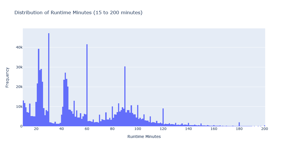

Distribution of Run-times in IMDB Dataset for items with runtimes between 10 and 200 minutes

Since IMDB Dataset has many different run-times, we can group them based on that. Also, since the range of numbers is quite long, we can shorten it into quarter minutes.

# Visualize all runtimes as quarters and grouped by media type
grouped_df = media_df.assign(runtimeQuarter=media_df['runtimeMinutes'].dropna().apply(lambda minutes: int((minutes + 14) / 15))).groupby('titleType')['runtimeQuarter'].value_counts().unstack(fill_value=0)

# Rename column names to show range
new_column_names = {col: f"{int(col)*15} to {int((col+1)*15)} minutes" for col in grouped_df.columns}
grouped_df.rename(columns=new_column_names, inplace=True)

fig = go.Figure()
for runtime_minutes in grouped_df.columns:
    fig.add_trace(go.Bar(x=grouped_df.index, y=grouped_df[runtime_minutes], name=str(runtime_minutes), customdata=['Col1', 'Col2', 'Col3']))
fig.update_traces(hovertemplate="%{y:.g} `%{x}` items")
fig.update_layout(barmode='stack', height=600, yaxis={'categoryorder': 'total descending'}, title='Media Runtime by Type', xaxis_title='Media Type', yaxis_title='Frequency')
fig.show()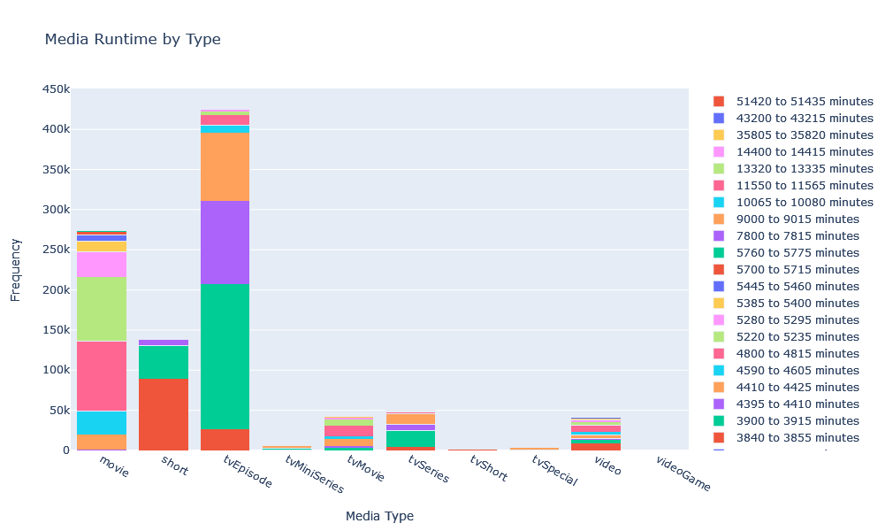

Run-times of media items in Quarter Minutes and Grouped by Media Type in IMDB DataSet

Investing the chart shows that most movies are between 90 to 105 minutes long, closly followed by movies between 105 to 120 minutes long. Also that most episodes are between 30 to 45 minutes long. Though, the interactive visualization of this chart(available in notebook) is much more easier to digest as there is too much information to show.

This type of chart is particularly useful to investigates anomalies. For example we can see that there are media items marked as short while being longer than 120 minutes.

Longest Runtime

Single media with longest runtime length:

runtime_top = media_df[media_df['runtimeMinutes']==media_df['runtimeMinutes'].max()]

Apparenty the documentary named “Logistics” with the runtime of 51420 minutes gets this title.

Alternativly, We can also take a look at top 10 media titles:

runtime_top_10_media = media_df.nlargest(10, 'runtimeMinutes')

Take note that first code was a condition to filter the media with max() function. the second code however used nlargest() function to filter items with largest values.

We can also combine conditions to filters. for example this code gets the movies with highest runtime:

runtime_top_10_movies = media_df[media_df['titleType'] == 'movie'].nlargest(10, 'runtimeMinutes')

And if want add a condition for a specific genres of movies, fo example comedy, we can do this:

runtime_top_10_movies_comedy = media_df[(media_df['titleType'] == 'movie') & (media_df['genres'].apply(lambda x: isinstance(x, list) and 'Comedy' in x))].nlargest(10, 'runtimeMinutes')

Note that apply() function has an addtional condition, isinstance(x, list), to check for the value type of genre to see if it’s a list. This will help avoide the items with no genres.

Year

Total number of movies per year in this chart shows a decline in the number of movies produces:

# Total number of movies per year
media_per_year = media_df['startYear'].dropna().value_counts().sort_index()[:-1] # current year is not included

fig = go.Figure(data=go.Scatter(x=media_per_year.index, y=media_per_year.values, mode='lines+markers'))
fig.update_layout(title_text='Number of Media Per Year', xaxis_title='Year', yaxis_title='Number of Media')
fig.show()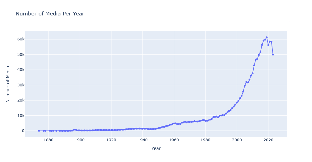

Number of Media Item Submitted to IMDB Per Year

First note that we skipped current year by adding [:-1] filter. This is because since this year is not yet finished, the chart can show a decline that is not representative of this year’s full activity.

Also this chart is only showing submitted media and is not a representative of how active different industries are. For that we need to analyze further features, as we can see later.

Genres and Year

Here we’ll be working with three features (media count, genre, and year) and display them on a 2D chart. First let’s get the total number of items for each genre, per year:

genre_year = media_df.explode('genres').groupby(['startYear', 'genres']).size().unstack(fill_value=0).astype(int)

And visualize it on a bar chart with different segments for each genre using add_trace() function:

fig = go.Figure()
for title_type in genre_year.columns:
    fig.add_trace(go.Bar(x=genre_year[title_type], y=genre_year.index, name=title_type, orientation='h'))
fig.update_layout(barmode='stack', yaxis={'categoryorder':'total descending'}, title='Published media by Start Year & Genre', xaxis_title='Number of media titles', yaxis_title='Genres')
fig.show()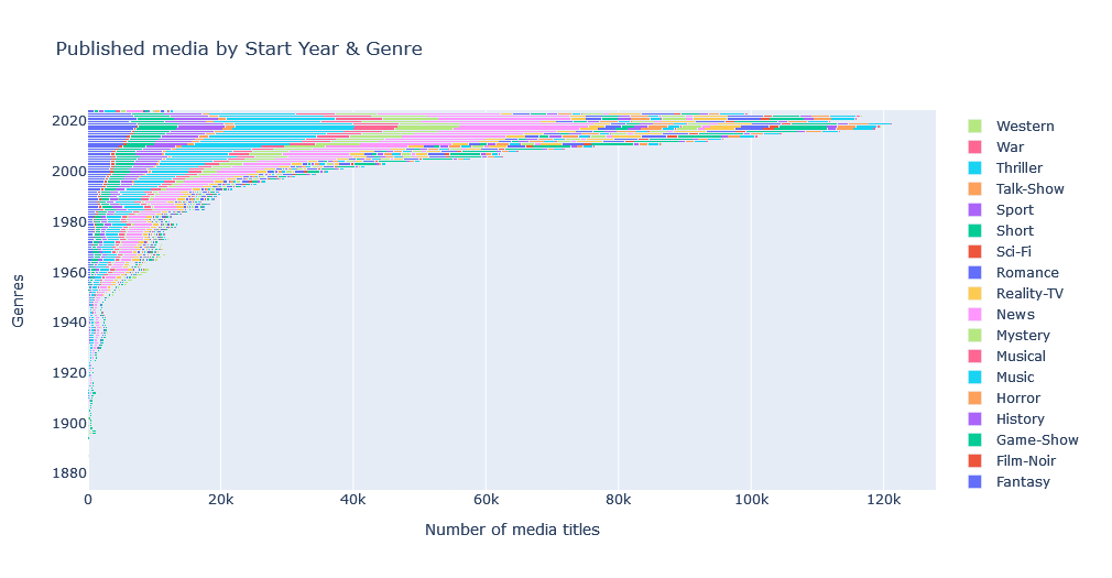

Published items on IMDB based on genre, over the years.

This interactive chart shows the number of title genres per year.

Genre and Type

Now let’s create a table for frequency of each genre for each media type, and visualize it:

grouped_df = media_df.explode('genres').groupby(['genres', 'titleType']).size().unstack(fill_value=0)

# Bar chart plot to visualize genres and segment them based on media type
fig = go.Figure()
for title_type in grouped_df.columns:
    fig.add_trace(go.Bar(x=grouped_df[title_type], y=grouped_df.index, name=title_type, orientation='h'))
fig.update_layout(barmode='stack', height=600, yaxis={'categoryorder':'total descending'}, title='Media Types Frequency by Genre', xaxis_title='Frequency', yaxis_title='Genres')
fig.show()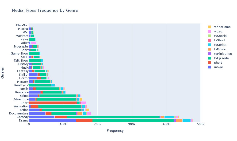

Checking the interactive chart and filtering media types by clicking on it’s legends, we can get more insights in distribution of genres for each media type. for example we can see that comedy is the most common genre for for TV series, yet most movies are dramas. Or we can zoom in a specific genre such as “musical” and see that most musicals are movies, followed by shorts.

Genre and Score

Instead of rating, let’s use previously calculated score and visualize it’s distribution over the years.

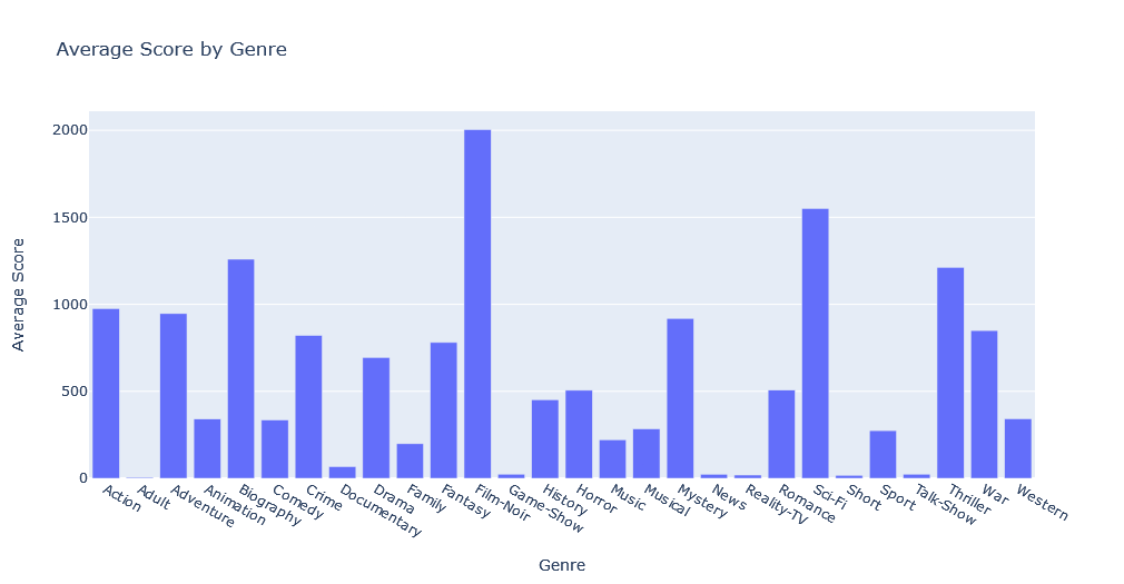
Average Score for Each Genre in IMDB Dataset

This bar chart shows that “Film-Noir” genre has the most hard-core fans, followed by Sci-Fi, Biographies, and Thrillers.

Rating over Year

Rating Count per Year

Now let’s take a look at number of votes cast each year in IMDB site.

total_votes_per_year = media_df.groupby('startYear')['numVotes'].sum().sort_index()[:-1] # Aggregate the total number of votes per year, ignoring last year

fig = go.Figure(data=go.Scatter(x=total_votes_per_year.index, y=total_votes_per_year.values, mode='lines+markers'))
fig.update_layout(title_text='Total Number of Votes Per Year', xaxis_title='Year', yaxis_title='Total Number of Casted Votes')

fig.show()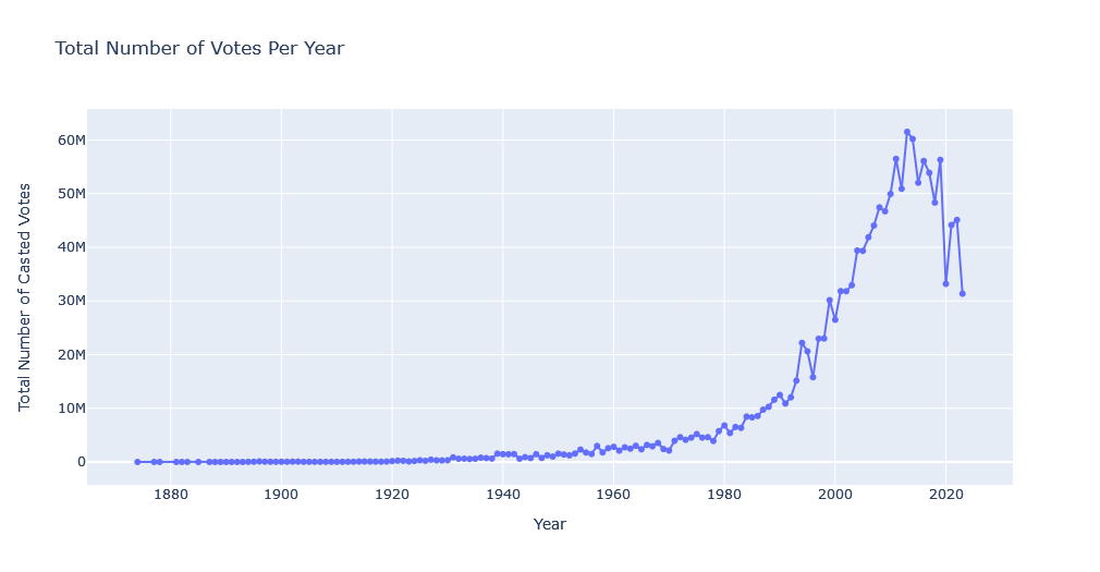

This data, rather than displaying the state of industry, displays the activity of IMDB users, with 2013 being peak of user voting in IMDB.

Average Rating per Year

Previous visualization displayed the voting counts. This scatter plot however, will visualize average rating of users by year:

grouped_ratings = media_df.groupby('startYear')['averageRating'].mean().reset_index()[:-1]

fig = go.Figure(data=go.Scatter(x=grouped_ratings['startYear'], y=grouped_ratings['averageRating'], mode='lines'))
fig.update_layout(title='Average Rating by Year', xaxis_title='Year', yaxis_title='Average Rating')

fig.show()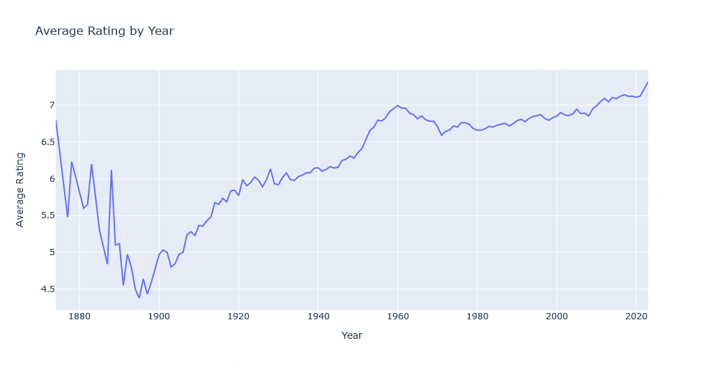

Average Rating of Media by IMDB Users over the Years

The sharp fall in years before 1900 is not normal. So we should further investigate it by drawing a more complex interactive chart with number of votes and number of media; as these features greatly influence distributions of ratings.

# Scatter plot for camparing average rating with number of votes and number of media published each year.
grouped_data = media_df.groupby('startYear').agg({'averageRating':'mean', 'numVotes':'sum', 'titleType':'count'}).reset_index()[:-1]
grouped_data = grouped_data.rename(columns={'titleType':'numMedia'})

fig = make_subplots(rows=1, cols=1)
fig = make_subplots(rows=1, cols=1, specs=[[{"secondary_y": True}]])

fig.add_trace(go.Scatter(x=grouped_data['startYear'], y=grouped_data['averageRating'], mode='lines', name='Average Rating', yaxis="y1"), secondary_y=False)
fig.add_trace(go.Scatter(x=grouped_data['startYear'], y=grouped_data['numVotes'], mode='lines', name='Number of Votes', yaxis="y2"))
fig.add_trace(go.Scatter(x=grouped_data['startYear'], y=grouped_data['numMedia'], mode='lines', name='Number of Media', yaxis="y3"))

fig.update_layout(title="Metrics Over the Years", xaxis_title="Year", hovermode="x unified",
                  xaxis=dict(
                      domain=[0.0, 0.85]
                  ),
                  yaxis=dict(title_text="Average Rating"),
                  yaxis2=dict(title_text="Number of Votes", overlaying="y",side="right", autoshift=True),
                  yaxis3=dict(title_text="Number of Media",overlaying="y",side="right", position=0.85, autoshift=True),
                  )
fig.show()

Various Metrics Over the Years, including average votes, number of votes, and number of media items.

This chart shows that the number of media items in years prior to 1930 is bellow a thousand. Given the small sample size, it’s generally unwise to use them to get insights from dataset.

Runtime over year

Now let’s take a look at average runtime of media items over the years via a simple bar chart:

average_runtime_per_year = media_df.groupby('startYear')['runtimeMinutes'].mean()

fig = go.Figure(data=go.Bar(x=average_runtime_per_year.index, y=average_runtime_per_year.values))
fig.update_layout(title_text='Average Runtime per Year', xaxis_title='Year', yaxis_title='Average Runtime (minutes)')
fig.show()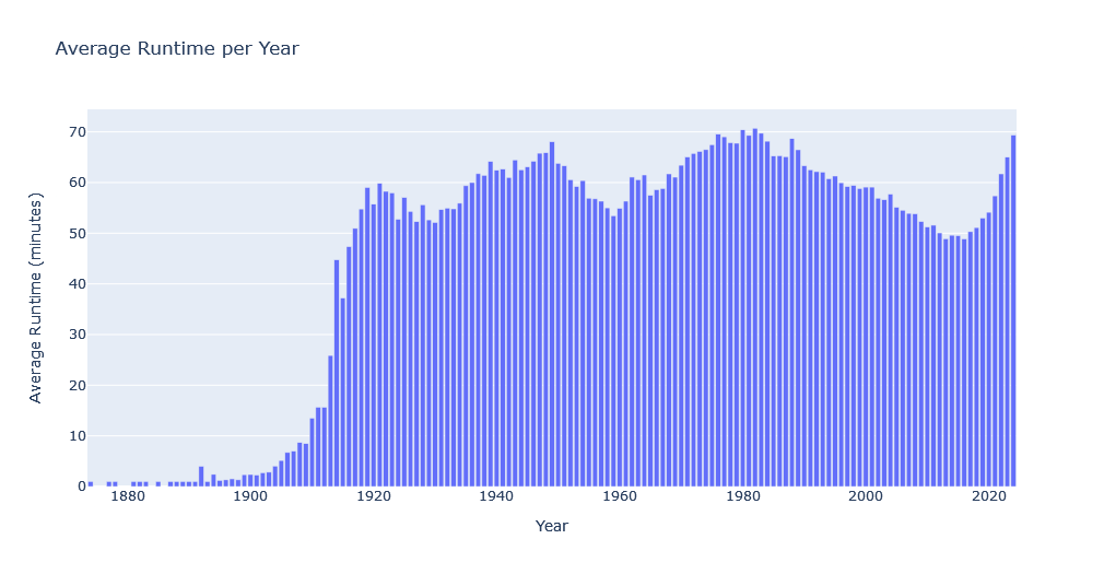

Average Runtime of media file in IMDB dataset per year

Not very interesting, is it. Instead let’s visualize average Runtime per year by media type:

average_runtime_by_type = media_df.groupby(['startYear', 'titleType'])['runtimeMinutes'].mean().unstack()

fig = go.Figure()
for title_type in average_runtime_by_type.columns:
    fig.add_trace(go.Bar(x=average_runtime_by_type.index, y=average_runtime_by_type[title_type], name=title_type))
fig.update_layout(barmode='stack', title_text='Average Runtime per Year by Title Type', xaxis_title='Year', yaxis_title='Average Runtime (minutes)')

fig.show()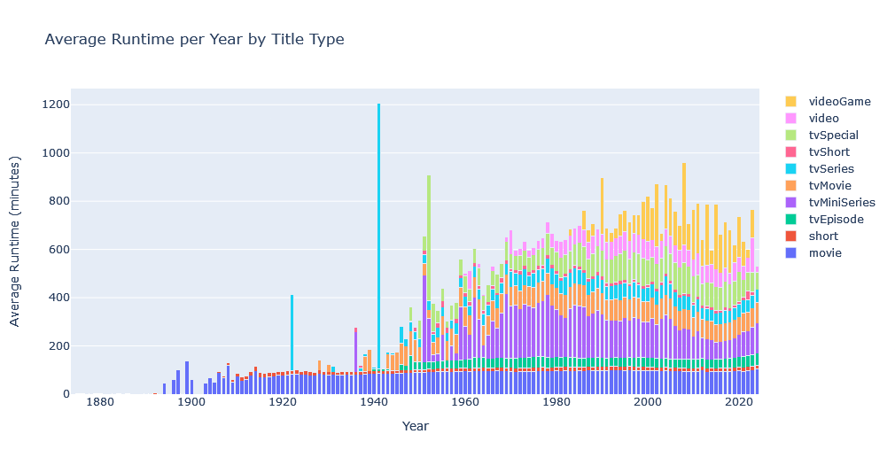

Average runtime of data items, per year for each media type

The spike for TV series runtime length in 1922 and 1941 in previous chart seems abnormal. Let’s investigate:

# TV Series in 1922 and 1922
tv_series = media_df[((media_df['titleType'] == 'tvSeries') & ((media_df['startYear'] == 1941) | (media_df['startYear'] == 1922)))]

The result explains the outline as it shows only 1 TV series for the years 1941 and 1922 with a runtime length that much higher than average:

 	tconst 	titleType 	primaryTitle 	originalTitle 	isAdult 	startYear 	endYear 	runtimeMinutes 	genres 	directors 	writers 	averageRating 	numVotes 	score
615410 	tt12950168 	tvSeries 	Canadian Army Newsreel 	Canadian Army Newsreel 	False 	1941 	1946 	1099 	[Documentary, News, War] 	NaN 	NaN 	3.9 	12 	-4.266666
1402395 	tt9642968 	tvSeries 	Vasaloppet 	Vasaloppet 	False 	1922 	<NA> 	314 	[Sport] 	NaN 	NaN 	6.8 	6 	1.733334

This shows the importance of sample size in statistical analysis.

Media Names (AKAs)

This file show the names given to specific titles based on region and language. Let’s list top 10 media items with highest number of title names:

aka_counts = aka_df['titleId'].value_counts().reset_index()
aka_counts.columns = ['titleId', 'count']
aka_counts['count'] = aka_counts['count'].astype('int16')
aka_counts.sort_values(by='count', ascending=False).head(10)

merged_df = media_df.merge(aka_counts, how='left', left_on='tconst', right_on='titleId')
top_10_media = merged_df.sort_values(by='count', ascending=False)
display(top_10_media.head(10))

Interestingly most of this titles, including all top 5 items, are animated series which shows that children shows have a higher global reach.

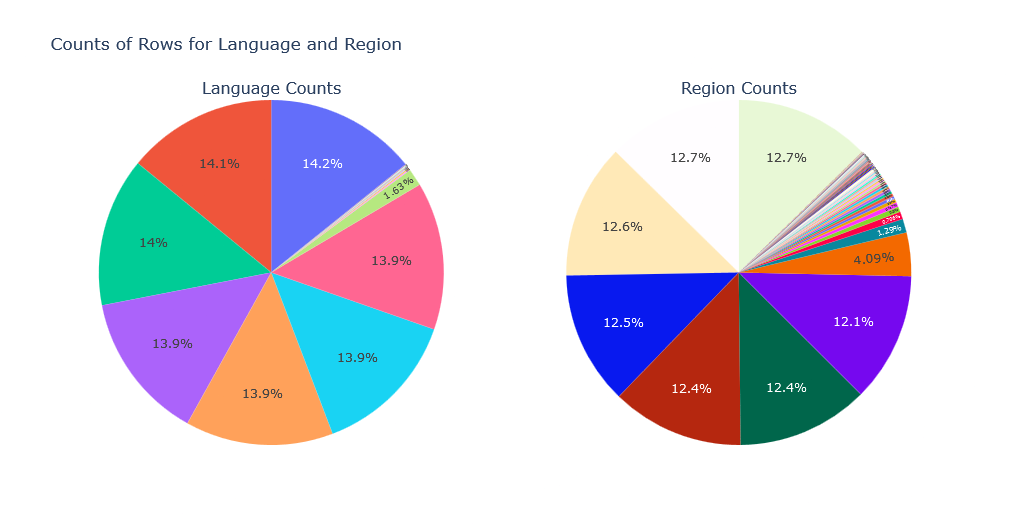
Now let’s see how alternative titles are distributed for regions and language:

language_counts = aka_df['language'].value_counts()
region_counts = aka_df['region'].value_counts()

fig = make_subplots(rows=1, cols=2, specs=[[{'type':'domain'}, {'type':'domain'}]], vertical_spacing=0.5, subplot_titles=("Language Counts", "Region Counts"))
fig.add_trace(go.Pie(labels=language_counts.index, values=language_counts.values, name="Language Counts", textposition = 'inside'), row=1, col=1)
fig.add_trace(go.Pie(labels=region_counts.index, values=region_counts.values, name="Region Counts", textposition = 'inside'), row=1, col=2)
fig.update_layout(title_text="Counts of Rows for Language and Region", showlegend=False)
fig.show()

Checkout interactive version of this chart for easier exploration of results.

Region and Language Distribution of AKA Titles in IMDB Dataset

TV Episodes

Now we shall explore TV Episodes. First we’ll create a histogram to visualize the distribution of TV episodes:

# Count episodes for each tv series
filtered_counts = episode_df['parentTconst'].value_counts()
filtered_counts = filtered_counts[filtered_counts < 300]

# Create a histogram to visualize the distribution of TV episodes
fig = go.Figure()
fig = go.Figure(data=[go.Histogram(x=filtered_counts, marker_color='skyblue')])
fig.update_layout(title_text='Distribution of TV Episodes (less than 300)', xaxis_title='Number of Episodes', yaxis_title='Frequency')

fig.show()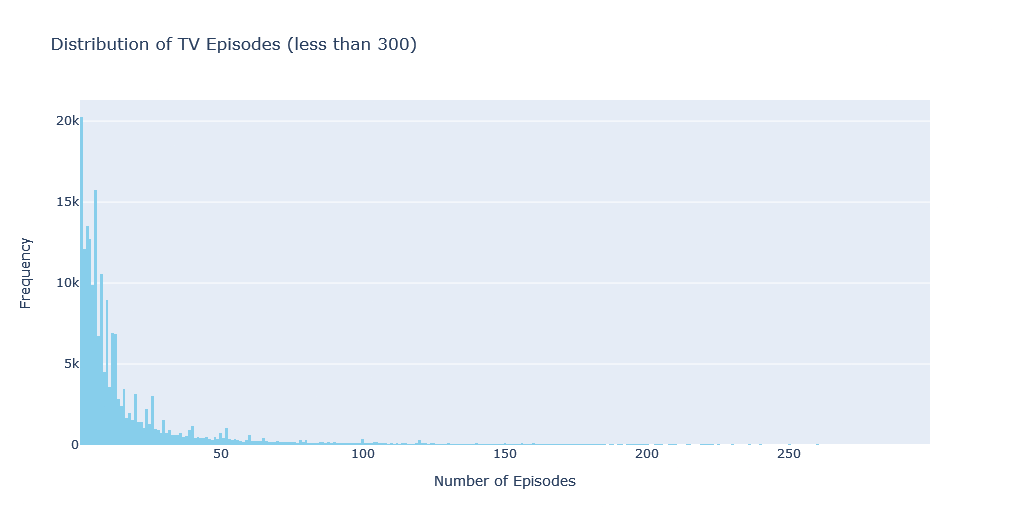

Distribution of Number of Episodes in TV Series in IMDB Dataset

To make the visualization more visible, tv series with more than 300 episodes are ignored. Note that if you are going to present an interactive chart to those who know how to explore it, you can visualize everything. but in image format this chart would not be usable.

Seeing this chart, we can see that there are many series with very few episodes, including just one episodes. This is because of pilot episodes and trial series. The rest shows that having series with 6, 8, 10, 12, and 13 episodes is more common.

Now we can can count the number of seasons and episodes for each TV series by counting unique seasons numbers and total number of episodes:

# Calculate the total count of seasons for each TV Series
number_of_seasons = episode_df.groupby('parentTconst')['seasonNumber'].nunique().reset_index()
number_of_seasons.columns = ['parentTconst', 'numberOfSeasons']

# Calculate the total count of episodes for each TV series
total_episodes = episode_df.groupby('parentTconst').size().reset_index()
total_episodes.columns = ['parentTconst', 'totalEpisodes']

# Merge the number of seasons and total episodes data
merged_data = number_of_seasons.merge(total_episodes, on='parentTconst')
# Merge with media_df to obtain the TV series name and other information
merged_data = merged_data.merge(media_df, left_on='parentTconst', right_on='tconst')

This code gives us access to number of season and episode count for each series, then merges it with the dataframe containing all the titles. Now we can perform more explorations. For example, show top 10 TV series with highest number of seasons:

series_most_seasons = merged_data.sort_values(by='numberOfSeasons', ascending=False).head(10)

As you can see in the results, “House Hunters” with 235 seasons and 3124 episodes gets the crown, followed by “House Hunters International”.

Now let’s check out the TV Series with highest number of episodes:

series_most_episodes = merged_data.sort_values(by='totalEpisodes', ascending=False).head(10)

Norwegian news show “NRK Nyheter” with 18593 total episodes(at the time of analysis, as the show is ongoing) is on the top of the list, followed by “Days of Our Lives” TV series with 14884 episodes in second place.

Writers, Directors, Crew

To get insights from list of directors and writers, let’s first prepare list of directors and writers of movies, and how many movies they worked on:

# list all directors and writers for "movies" and get their name, and how many movies they wrote or directed
directed_count = media_df[media_df['titleType'] == 'movie']['directors'].explode().value_counts().reset_index().rename(columns={'index':'nconst', 'directors':'directed_count'})
wrote_count = media_df[media_df['titleType'] == 'movie']['writers'].explode().value_counts().reset_index().rename(columns={'index':'nconst', 'writers':'wrote_count'})

# Merge the counts with the name_df dataframe to get the real names and additional information
directed_and_wrote_count = directed_count.merge(wrote_count, on='nconst', how='outer')
directed_and_wrote_count = directed_and_wrote_count.merge(name_df, on='nconst', how='left')

directed_and_wrote_count.fillna(0, inplace=True)
directed_and_wrote_count[['directed_count', 'wrote_count']] = directed_and_wrote_count[['directed_count', 'wrote_count']].astype(int)

and get 10 most prolific movie directors:

directed_and_wrote_count.sort_values(by='directed_count', ascending=False).head(10)

and top 10 most prolific movie writers:

directed_and_wrote_count.sort_values(by='wrote_count', ascending=False).head(10)

This is an interesting list. Sam Newfield is the most prolific movie director with 204 movies. And so far 412 movies were adopted from the works of William Shakespeare, making him the most prolific movie writer.

Sorting writers based on their birthday shows oldest writers whose work was adopted as movies:

oldest_writers = directed_and_wrote_count[directed_and_wrote_count['birthYear'] != 0].sort_values(by='birthYear', ascending=True).head(10)

Now let’s look at the longest lived writers and directors:

directed_and_wrote_count['lifespan'] = directed_and_wrote_count.apply(lambda row: row['deathYear'] - row['birthYear'] if row['birthYear'] != 0 else 0, axis=1)
longest_lived_individuals = directed_and_wrote_count.nlargest(10, 'lifespan')

This record belongs to Fakir Lalon Shah who lived for 118 years as he is attributed as a writer for a movie, followed by Frederica Sagor Maas who lived for 112 years and had 13 of his works adopted into movies.

Conclusion

This post has taken you through a step-by-step Exploratory Data Analysis (EDA) of the IMDB dataset. We explored the structure of various data files, delved into reading and understanding the data using Pandas, and discussed strategies for obtaining summary statistics and exploring the data visually.

IMDB Dataset is quite rich and this EDA has just scratched the surface of the rich information available within the IMDB dataset. What insights were most interesting to you? Are there any specific data explorations you’d like to see next? Feel free to leave a comment and share your thoughts!